Exploring coupled images fusion based on joint tensor decomposition

Abstract

Data fusion has always been a hot research topic in human-centric computing and extended with the development of artificial intelligence. Generally, the coupled data fusion algorithm usually utilizes the information from one data set to improve the estimation accuracy and explain related latent variables of other coupled datasets. This paper proposes several kinds of coupled images decomposition algorithms based on the coupled matrix and tensor factorization-optimization (CMTF-OPT) algorithm and the flexible coupling algorithm, which are termed the coupled images factorization-optimization (CIF-OPT) algorithm and the modified flexible coupling algorithm respectively. The theory and experiments show that the effect of the CIF-OPT algorithm is robust under the influence of different noises. Particularly, the CIF-OPT algorithm can accurately restore an image with missing some data elements. Moreover, the flexible coupling model has better estimation performance than a hard coupling. For high-dimensional images, this paper adopts the compressed data decomposition algorithm that not only works better than uncoupled ALS algorithm as the image noise level increases, but saves time and cost compared to the uncompressed algorithm.

Introduction

Image data fusion has been a hot research topic in neuroscience, metabonomics and other fields, and has been widely used in real life. The coupled data fusion algorithm usually utilizes the information of one data set to improve the estimation accuracy and the interpretation of related potential variables of other data sets. With the development of electronic and imaging technology, it is difficult to find accurate data for digital images for human beings, such as medical science [1], information remote sensing and so on. In this situation, people hope to primitively analyze mass images and select the information quickly and effectively by more convenient calculation way. Moreover, traditional data processes mechanisms are less efficient when faced with large amounts of data in human-centric computing. And we apply the tensor structures to represent massive data to solve above problems in this paper because of its multi-dimensional property.

Multi-source image data fusion refers to making the comprehensive image analysis for the image data obtained from different acquisition devices (known as multi-source heterogeneous image data), so as to achieve complementary information from different information sources, and finally obtain clearer, more informative and higher quality fused images. It is that we can use different types of electronic data collection sensors to manage, analyze and integrate resources efficiently to provide clearer images to humans. However, multi-source heterogeneous image data analysis is now facing many problems. Complex data objects have multiple dimensions, and how to depict the relationship between them through data analysis is one of the challenges to solve urgently.

For example, we cannot utilize a general matrix to express the spectral image as there are multiple spectral band, (e.g. the mode 3 axis), where each spectral band represents a color image matrix. And we can see that multi-channel images have natural tensor structures from the above case. Moreover, the superposition of image matrix can be seen as a video if the mode 3 axis represents time, and above two tensor structures are shown in Figs. 1 and 2. Therefore, tensor can express multiple relationships in the real world, while this paper studies image fusion based on tensor analysis, which can abstractly describe the interaction mechanism between multiple aspects of image data. In addition, tensor structure has strong expression ability and computational properties, so it is very meaningful to study tensor analysis of images. Tensor decomposition is a very significant knowledge content, which can preserve the structural characteristics of the original image data [2].

Fig. 1

The tensor structure of the multispectral image

Fig. 2

The tensor structure of the video

What’s more, multi-source heterogeneous semantics are much more rich. How to build a generalization model that integrates multi-source data or discover the correlation between them is another challenge for multi-source heterogeneous images. In this paper, we generally use couplings to refer to the correlation between heterogeneous images. When doctors make the diagnosis for a patient’s brain, they can get some images of the patient’s brain from a variety of ways, as shown in Fig. 3. And whether there is a coupling between these brain images, and how to combine them to determine the etiology of patients are the questions to be discussed in this paper. In addition, for the fusion of hyperspectral images and multispectral images, the purpose is to fuse the information in the same scene to generate fusion image with large amount of information and high quality, as shown in Fig. 4. Similarly, what is the correlation between the information contained in these spectral images and how to combine complementary information to get a clearer image is also the significance of this paper.

Fig. 3

The diagnosis process for a patient’s brain

Fig. 4

The task diagram of hyperspectral hyper-resolution

The outline of this paper is organized as follows. In “Related work” section, related work about coupled images fusion is discussed. And we mainly describe some basic notations and definitions on tensors in “Tensor and related notation” section. In “Coupled image fusion” section, the proposed coupled image fusion algorithms are presented. Moreover, the experimental results on algorithms are shown in “Experiments and results” section. Finally, we give some conclusions and future research directions we need to study next.

Related work

Recently, motivated by the tensor nuclear norm(TNN), Pan Zhou and Canyi Lu proposed a novel low-rank tensor factorization method for efficiently solving the 3-way tensor completion problem, which can recover the synthetic data, inpainting images and videos with superior performance and efficiency [3]. For hyperspectral images, tensor decomposition can make full use of space and inter spectral redundancy between images, compressing the high spectral image and extracting the related feature information fast and high-quality [4,5,6]. Chia-Hsiang Lin et al proposed a convex optimization-Based coupled nonnegative matrix factorization algorithm for hyperspectral and multispectral data fusion [7]. Li and Dian proposed a coupled sparse tensor factorization (CSTF)-based approach for fusing hyperspectral images and multispectral images to obtain a high spatial resolution hyperspectral image [8]. In addition, they consider high spatial resolution hyperspectral image (HR-HSI) as a 3D tensor and redefine the fusion problem as the estimation of a core tensor and dictionaries of the three modes [9]. Veganzones and Cohen proposed a Canonical Polyadic decomposition (CP) algorithm based on hyperspectral images, which was used to solve the problem of blind source signal separation [4]. They suggested to solve this problem as a low dimensional constrained tensor decomposition and applied kinds of fast decomposition of large nonnegative tensors which allowed a major speed up in the computation of the decomposition [10].

In the past few years, there have been many researches on the application of CP decomposition in image. In [11, 12] used the CP decomposition into image compression and classification. Marcella Astrid et al used the CP decomposition into Convolutional Neural Networks (CNNs) to solve the image classification tasks [13]. Bauckhage introduced discriminant analysis to higher order data(i.e. color images) for classification [14]. For hyperspectral and multispectral images (i.e. multi-source heterogeneous data), kinds of methods exploits the Bayesian framework [15,16,17] to fuse such images. Rodrigo and Jeremy proposed a Bayesian framework to define flexible coupling models for joint tensor decompositions of multiple datasets [18, 19]. They cast the problem of data fusion as the analysis of latent variable. And the latent models between data are coupled through subsets of their variables, where the coupling refers to the relationship between these variables subset. That is, there is a coupling relationship between the factor matrix after the tensor decomposition. In this paper, we hope to use the coupling relation between images to solve the problem, improving the accuracy and interpretability of the latent variables related to the other data set from the information of one data set through joint tensor decomposition algorithm.

In application, data analysis from different data sources needs to be handled the heterogeneous datasets (i.e. a matrix or a high-order tensor) [20, 21]. Recently, matrix factorization and tensor-based factorization have been successfully applied to multi-frame data restoration [22,23,24,25], recognition [26, 27], unmixing [28] and data fusion [18], etc. For the data analysis of some coupled matrices and tensors, corresponding coupled matrix and tensor factorization-optimization algorithm (i.e. CMTF-OPT) was proposed in [29]. The numerical experiments showed that The CMTF algorithm had better performance than CP algorithm in data recovery at a certain level of noise.

Similarly, the higher order coupled tensor decomposition problem was also studied in [10]. Model showed better performance in coupled tensor decomposition in the experiments. Rodrigo and Jérémy studied the coupling relationship between different data and the data decomposition algorithms under coupling, which showed that the decomposition algorithm based on coupled data had better convergence and the calculation of the algorithm took less time than alternating least squares (ALS) algorithm [18]. So using the coupling relations between images is the necessary measure and work to decompose images. Moreover the algorithms in [18, 29] are not used to the coupled images. And S. Li and R. Dian do not make full use of the coupling relationship between images and use this coupling relation to accelerate the operation of the algorithm and restore the coupled image data [8]. Therefore, this paper proposes the coupled image data decomposition algorithms based on the CMTF-OPT algorithm [29] and the coupled tensor data decomposition algorithm [18].

Tensor and related notation

In the nineteenth century, Gauss and Riemann put forward the concept of tensors in the study of differential geometry. In 1916, Einstein applied tensors to the study of the general relativity, which made tensor analysis to be an important tool in continuum mechanics, theoretical physics and other disciplines. In 2005, characteristic polynomial was proposed for the first time in real symmetric tensor by Qi, and he presented the definition of the eigenvalues [30].

In order to study the data fusion between the coupled images better and simplify the presentation, this paper first introduces some of the following symbols and definitions. For the general tensor, this paper uses the calligraphic letters to represent them e.g. ${\mathcal {X}}$, the matrix is denoted by capital letters e.g. ${{\mathbf {X}}}$, and the scalar (or. vector) is represented by lowercase, e.g. x. The mode-n matricization of a tensor ${\mathcal {X}}\in {\mathbb {R}}^{I_{1}\times I_{2}\times \cdots \times I_{N}}$ is denoted by ${\mathcal {X}}_{(n)}$, which can reduce the dimension of the tensor. For a matrix ${{\mathbf {A}}}\in {\mathbb {R}}^{I\times J}$, vectorization is to expand the matrix by column, forming a IJ Column vector, that is

$$\begin{aligned} {\mathrm {vec}}({{\mathbf {A}}})=\left[ \begin{array}{c} a_{1}\\ \vdots \\ a_{J}\\ \end{array} \right] \in {\mathbb {R}}^{IJ}. \end{aligned}$$

(1)

Given two matrices ${{\mathbf {A}}}\in {\mathbb {R}}^{I\times K}$ and ${{\mathbf {B}}}\in {\mathbb {R}}^{J\times K}$, the Khatri-Rao product is denoted as ${{\mathbf {A}}} \odot {{\mathbf {B}}}$, and the calculation results is a matrix of size $IJ\times K$ and defined by

$$\begin{aligned} {{\mathbf {A}}}\odot {{\mathbf {B}}}=[a_{1}\otimes b_{1}\quad a_{2}\otimes b_{2} \quad \cdots \quad a_{K}\otimes b_{K}] , \end{aligned}$$

(2)

where $\otimes$ is the Kronecker product.

Given two tensors ${\mathcal {A}},{\mathcal {B}}\in {\mathbb {R}}^{I_{1}\times I_{2}\times \cdots \times I_{N}}$, the Hadamard product denoted as ${\mathcal {A}}*{\mathcal {B}}$, and the calculation results is a matrix of size $I\times J$, i.e.

$$\begin{aligned} {\mathcal {A}}*{\mathcal {B}}=\left[ \begin{array}{cccc} a_{11}b_{11}&{}a_{12}b_{12}&{}\cdots &{}a_{1J}b_{1J}\\ a_{21}b_{21}&{}a_{22}b_{22}&{}\cdots &{}a_{2J}b_{2J}\\ \vdots &{}\vdots &{}\ddots &{}\vdots \\ a_{I1}b_{I1}&{}a_{I2}b_{I2}&{}\cdots &{}a_{IJ}b_{IJ}\\ \end{array} \right] . \end{aligned}$$

(3)

Given two tensors ${\mathcal {A}},{\mathcal {B}}\in {\mathbb {R}}^{I_{1}\times I_{2}\times \cdots \times I_{N}}$,the inner product is defined as the sum of the product of its elements, i.e.

$$\begin{aligned} \langle {\mathcal {A}},{\mathcal {B}}\rangle =\sum \limits _{i_{1}=1}^{I_{1}}\sum \limits _{i_{2}=1}^{I_{2}}\cdots \sum \limits _{i_{N}=1}^{I_{N}} {x_{i_{1}i_{2}\cdots i_{N}}y_{i_{1}i_{2}\cdots i_{N}}}, \end{aligned}$$

(4)

we usually use ’$\circ$’ to represent the outer product.

Let matrix ${{\mathbf {A}}}=(a_{ij})_{m\times n}\in {\mathcal {C}}^{m\times n}$, the Frobenius norm is defined as

$$\begin{aligned} \parallel {{\mathbf {A}}} \parallel _{{\mathrm {F}}}=\left( \sum _{i=1}^{m}\sum _{j=1}^{n}|a_{ij}|^{2}\right) ^{\frac{1}{2}}. \end{aligned}$$

(5)

Tensor decomposition

In applications, the general tensor decomposition models can be divided into two categories, which are the Canonical Polyadic/PARAFAC decomposition (e.g. CP decomposition) and the Tucker decomposition model. The canonical decomposition was originally proposed by Carroll and Chang [31] and PARAFAC (parallel factors) by Harshman [32] separately. In 1966 Tucker [33] proposed the Tucker model. In particular, the CP decomposition model is a special case of the Tucker decomposition model. At the time, models were put forward to extract data characteristics from psychological tests. For the general matrix model, we can extract the potential information of matrix data, such as hyperspectral data fusion and blind source separation, by means of singular value decomposition of matrix, nonnegative matrix decomposition and so on. Similar to the idea of low rank approximation of matrix, researchers also want to extract latent information from tensor model data by means of tensor decomposition model.

For a tensor ${\mathcal {X}}\in {\mathbb {R}}^{I_{1}\times I_{2}\times \cdots \times I_{N}}$, the CP decomposition is expressed as

$$\begin{aligned} {\mathcal {X}}\approx \sum \limits _{r=1}^{R}\lambda _{r}a_{r}^{(1)}\circ a_{r}^{(2)}\circ \cdots \circ a_{r}^{(N)} = \llbracket \lambda ;{{\mathbf {A}}}^{(1)},{{\mathbf {A}}}^{(2)},\ldots ,{{\mathbf {A}}}^{(N)} \rrbracket , \end{aligned}$$

(6)

where R is a positive integer, ${{\mathbf {A}}}^{(n)}$ is called the factor matrix, which is a combination of rank one vector $a_{r}^{(n)}$, e.g.

$$\begin{aligned} {{\mathbf {A}}}^{(n)}=[a_{1}^{(n)},a_{2}^{(n)},\ldots ,a_{R}^{(n)}], \end{aligned}$$

(7)

for $n=1,2,\ldots ,N$, $\lambda \in {\mathbb {R}}^{R}$, $a_{r}^{(n)}\in {\mathbb {R}}^{I_{n}}$, ${{\mathbf {A}}}^{(n)}\in {\mathbb {R}}^{I_{n}\times R}$.

Especially, for the three order tensor ${\mathcal {X}}\in {\mathbb {R}}^{I \times J \times K}$, the CP decomposition is expressed as

$$\begin{aligned} {\mathcal {X}}\approx \sum \limits _{r=1}^{R}\lambda _{r}a_{r}\circ b_{r}\circ c_{r} = \llbracket \lambda ;{{\mathbf {A}}},{{\mathbf {B}}},{{\mathbf {C}}} \rrbracket , \end{aligned}$$

(8)

where $r=1,2,\cdots ,R$, $\lambda \in {\mathbb {R}}^{R}$, $a_{r}\in R^{I}$, $b_{r}\in R^{J}$, $c_{r}\in R^{K}$.

Here, the column of factor matrix ${{\mathbf {A}}}$, ${{\mathbf {B}}}$ and ${{\mathbf {C}}}$ is normalized to 1, and $\lambda _{r}$ is the weight. If the weight is assigned to the factor matrix, the CP decomposition can also be showed as

$$\begin{aligned} {\mathcal {X}}\approx ({{\mathbf {A}}}^{'},{{\mathbf {B}}}^{'},{{\mathbf {C}}}^{'}). \end{aligned}$$

(9)

Now we define ${\mathcal {D}}_{r}$ composed of $\lambda _{r}$ is $R\times R\times R$ order diagonal tensor, so the equation can be transformed into

$$\begin{aligned} {\mathcal {X}}=({{\mathbf {A}}},{{\mathbf {B}}},{{\mathbf {C}}})\cdot {\mathcal {D}}_{r}. \end{aligned}$$

(10)

Coupled image fusion

Coupled data fusion

Data fusion, also known as collective data analysis, has been a hot topic in different fields. Data analysis from multiple sources has attracted considerable people in the Netflix Grand Prix. The goal is to accurately predict movie ratings. In order to get better ratings, additional data sources supplement the user score, such as the label information has been used. And the collective matrix factorization (CMF) proposed by Singh and Gordon [34] is based on the correlation between data sets, and the coupling matrix is factored simultaneously. Many researchers have paid their more attention to image fusion technique based on pulse coupled neural network. Literature [35] described the models and modified ones. As to the multi-focus image fusion problem, Veshki et al. utilized the sparse representation using a coupled dictionary to address the focused and blurred feature problem for higher quality [36]. In order to create spectral images with high spectral and spatial resolution, Yuan Zhou et al [37] proposed a fusion algorithm by combining linear spectral unmixing with the local low-rank property by extracting the abundance and the endmembers of Hyperspectral images usually have high spectral and low spatial resolution. Conversely, multispectral images.

For two matrices ${{\mathbf {X}}}\in {\mathbb {R}}^{I\times M}$, ${{\mathbf {Y}}}\in {\mathbb {R}}^{I\times L}$, the general CMF decomposition model is established by minimizing the following objective function

$$\begin{aligned} f({{\mathbf {U}}},{{\mathbf {V}}},{{\mathbf {W}}})=\parallel {{\mathbf {X}}}-{{\mathbf {U}}}{{\mathbf {V}}}^{{\mathrm {T}}}\parallel _{{\mathrm {F}}} ^{2}+\parallel {{\mathbf {Y}}}-{{\mathbf {U}}}{{\mathbf {W}}}^{{\mathrm {T}}}\parallel _{{\mathrm {F}}} ^{2}, \end{aligned}$$

(11)

where the matrices ${{\mathbf {U}}}\in {\mathbb {R}}^{I\times R}$, ${{\mathbf {V}}}\in {\mathbb {R}}^{M\times R}$ and ${{\mathbf {W}}}\in {\mathbb {R}}^{L\times R}$ are the factor matrices, R is the number of factors. In particular, because there exists a large number of high-order data, the data fusion between the coupled tensor and the matrix is discussed below.

For a tensor ${\mathcal {X}}\in {\mathbb {R}}^{I\times J\times K}$ and a matrix ${{\mathbf {Y}}}\in {\mathbb {R}}^{I\times M}$, the general coupled tensor and matrx decomposition model is established by modifying the above objective function

$$\begin{aligned} f({{\mathbf {A}}},{{\mathbf {B}}},{{\mathbf {C}}},{{\mathbf {V}}})=\parallel {\mathcal {X}}-({{\mathbf {A}}},{{\mathbf {B}}},{{\mathbf {C}}})\parallel _{{\mathrm {F}}}^{2}+\parallel {{\mathbf {Y}}}-{\mathbf {AV}}^{T}\parallel _{{\mathrm {F}}} ^{2}, \end{aligned}$$

(12)

where the matrices ${{\mathbf {A}}}\in {\mathbb {R}}^{I\times R}$, ${{\mathbf {B}}} \in {\mathbb {R}}^{J\times R}$ and ${{\mathbf {C}}}\in {\mathbb {R}}^{K\times R}$ are factor matrices obtained by CP decomposition of the tensor ${\mathcal {X}}$.

Alternating Least Squares Algorithm for coupled matrix and tensor factorization (CMTF-ALS) algorithm is proposed in [29]. The algorithm based on ALS is simple, small and effective. However, the convergence of the algorithm based ALS is not good with the missing data [38]. On the other hand, it is more robust to solve all CP factor matrices with an optimized algorithm, and is more easily extended to the missing data set [39]. Therefore, for high order data sets, with the support of the algorithm proposed in [29], this paper presents some coupled image decomposition algorithms, which describe the coupling analysis of heterogeneous image data sets.

Coupled tensor decomposition algorithm

CIF-OPT algorithm

The main purpose of this paper is exploring data fusion between coupled images. In general, images are stored in terms of tensor or matrix. Based on the CMTF optimization (CMTF-OPT) algorithm in [29], a coupled images factorization-optimization(CIF-OPT) algorithm is proposed. We firstly consider matrix image and N-order tensor image with one mode in common, where tensor image is decomposed through CP model and matrix image is decomposed through matrix decomposition.

Given a tensor image ${\mathcal {X}}\in {\mathbb {R}}^{I_{1}\times I_{2}\times \cdots \times I_{N}}$ and a matrix image ${{\mathbf {Y}}}\in {\mathbb {R}}^{I_{1}\times M}$ which have the nth mode in common, where $n\in \{1,\ldots ,N\}$. Without loss of generality, we assume that two images coupled in the third mode, and the common latent structure in these images can be extracted by CIF-OPT algorithm. The objective function of the coupled analysis between the two image datasets is as follow

$$\begin{aligned} f({{\mathbf {A}}}^{(1)},{{\mathbf {A}}}^{(2)},\ldots ,{{\mathbf {A}}}^{(N)},{{\mathbf {V}}})=\parallel {\mathcal {X}}- \llbracket {{\mathbf {A}}}^{(1)},{{\mathbf {A}}}^{(2)},\ldots ,{{\mathbf {A}}}^{(N)} \rrbracket \parallel _{{\mathrm {F}}} ^{2} +\parallel {{\mathbf {Y}}}-{{\mathbf {A}}}^{(n)}V^{{\mathrm {T}}}\parallel _{{\mathrm {F}}} ^{2}, \end{aligned}$$

(13)

In order to solve the above optimization problem, we can calculate its gradient and solve it by using any first order optimization algorithm of [40]. Next, this paper will discuss the gradient of the objective function, the first item of the function (11) is written as

$$\begin{aligned} f_{1}=\parallel {\mathcal {X}}- \llbracket {{\mathbf {A}}}^{(1)},{{\mathbf {A}}}^{(2)},\cdots ,{{\mathbf {A}}}^{(N)} \rrbracket \parallel _{{\mathrm {F}}} ^{2}, \end{aligned}$$

(14)

the second item of the function (11) is recorded as

$$\begin{aligned} f_{2}=\parallel {{\mathbf {Y}}}-{{\mathbf {A}}}^{(n)}V^{{\mathrm {T}}}\parallel _{{\mathrm {F}}} ^{2}. \end{aligned}$$

(15)

Let ${\mathcal {S}}= \llbracket {{\mathbf {A}}}^{(1)},{{\mathbf {A}}}^{(2)},\ldots ,{{\mathbf {A}}}^{(N)} \rrbracket$,and the specific forms of the partial derivative of $f_{1}$ with respect to ${{\mathbf {A}}}^{(i)}$ are as below

$$\begin{aligned} \frac{\partial f_{1}}{\partial {{\mathbf {A}}}^{(i)}}=({{\mathbf {S}}}_{(i)}-{{\mathbf {X}}}_{(i)}){{\mathbf {A}}}^{(-i)}, \end{aligned}$$

(16)

where $i=1,2,\ldots ,N$.The matrices ${{\mathbf {A}}}$ and ${{\mathbf {V}}}\in {\mathbb {R}}^{M\times R}$are factor matrices obtained by matrix decomposition of the matrix ${{\mathbf {Y}}}$.

$$\begin{aligned} {{\mathbf {A}}}^{(-i)}={{\mathbf {A}}}^{(N)}\odot \cdots \odot {{\mathbf {A}}}^{(i+1)}\odot {{\mathbf {A}}}^{(i-1)}\odot {{\mathbf {A}}}^{(1)}. \end{aligned}$$

(17)

The specific forms of the partial derivative of $f_{2}$ with respect to ${{\mathbf {A}}}^{(i)}$ and ${{\mathbf {V}}}$ can be computed as

$$\begin{aligned} \frac{\partial f_{2}}{\partial {{\mathbf {A}}}^{(i)}}= \left\{ \begin{array}{l} -{\mathbf {YV}}+{{\mathbf {A}}}^{(-i)}{{\mathbf {V}}}^{{\mathrm {T}}}{{\mathbf {V}}}, \qquad \qquad for\;\;\; i=n,\\ 0,\qquad \qquad \qquad \qquad \qquad \qquad for \;\; i\ne n. \\ \end{array} \right. \end{aligned}$$

(18)

$$\begin{aligned} \frac{\partial f_{2}}{\partial {{\mathbf {V}}}}=-{{\mathbf {Y}}}^{{\mathrm {T}}}{{\mathbf {A}}}^{(i)}+{\mathbf {VA}}^{(i)^{{\mathrm {T}}}}{{\mathbf {A}}}^{(i)}. \end{aligned}$$

(19)

Combined with the above calculation results, we can calculate the objective function f.

$$\begin{aligned} \frac{\partial f}{\partial {{\mathbf {A}}}^{(i)}}=\frac{\partial f_{1}}{\partial {{\mathbf {A}}}^{(i)}}+\frac{\partial f_{2}}{\partial {{\mathbf {A}}}^{(i)}},\frac{\partial f}{\partial {{\mathbf {V}}}}=\frac{\partial f_{2}}{\partial {{\mathbf {V}}}}=-{{\mathbf {Y}}}^{{\mathrm {T}}}{{\mathbf {A}}}^{(i)}+{\mathbf {VA}}^{(i)^{{\mathrm {T}}}}{{\mathbf {A}}}^{(i)}. \end{aligned}$$

(20)

Finally, this paper calculates the gradient of the optimization function f, and its specific form is a vector e.g.

$$\begin{aligned} \nabla f= \left[ \begin{array}{c} {\mathrm {vec}}\left( \frac{\partial f}{\partial {{\mathbf {A}}}^{(1)}}\right) \\ \vdots \\ {\mathrm {vec}}\left( \frac{\partial f}{\partial {{\mathbf {A}}}^{(N)}}\right) \\ {\mathrm {vec}}\left( \frac{\partial f}{\partial {{\mathbf {V}}}}\right) \\ \end{array} \right] . \end{aligned}$$

(21)

where the length of the vector is $P=R\sum _{n=1}^N(I_{N}+M)$, which can be formed by vectorizing the partial derivatives with respect to each factor matrix and forming a column vector.

For some missing data sets, coupling analysis can still be carried out. The implementation of the algorithm can ignore missing data, and only analyze the known data elements to find the tensor or matrix model. And we applied it to the missing image and restored the original image based on the proposed coupled image decomposition algorithm through the another coupled image, which refer to [29].

Flexible coupling models

Rodrigo and Jérémy proposed the flexible coupling models based on the joint decomposition of Bayesian estimation in [18]. They mainly present two general examples of coupling priors such as joint Gaussian priors and non Gaussian conditional distributions. For two tensors with noisy measurements ${\mathcal {Y}}$ and ${\mathcal {Y}}^{'}$, ${\mathcal {Y}}$ is a second tensor (e.g. matrix) which can be the SVD ${\mathcal {Y}}={{\mathbf {U}}}{\varvec{\Sigma }} {{\mathbf {V}}}^{{\mathrm {T}}}+{{\mathbf {E}}}$, and ${\mathcal {Y}}^{'}$ is a third order tensor which can be written ${\mathcal {Y}}^{'}=({{\mathbf {A}}}^{'},{{\mathbf {B}}}^{'},{{\mathbf {C}}}^{'})+\varepsilon ^{'}$ via CP decomposition, where ${{\mathbf {E}}}$ and $\varepsilon ^{'}$ are the noisy array.

Let $\theta ={\mathrm {vec}}([{{\mathbf {U}}};{\varvec{\Sigma }};{{\mathbf {V}}}^{{\mathrm {T}}}])$ and $\theta ^{'}={\mathrm {vec}}({{\mathbf {A}}}^{'};{{\mathbf {B}}}^{'};{{\mathbf {C}}}^{'})$. Here we assume the parameters $\theta$ and $\theta ^{'}$ are random and consider that the coupling between them is flexible, for instance, we could have ${\mathbf {V=B}}$, or ${\mathbf {V=WB}}$ for a known transformation matrix ${{\mathbf {W}}}$. Under the some simplifying hypotheses underlying the Bayesian approach, the Maximum a posteriori estimator (MAP) estimator is given as the minimizer of the following cost function

$$\begin{aligned} \arg \min \limits _{\theta ,\theta ^{'}}\Upsilon (\theta ,\theta ^{'})=-\log p({\mathcal {Y}}\mid \theta )-\log p(\mathcal {Y^{'}}\mid \theta ^{'})-\log p(\theta ,\theta ^{'}). \end{aligned}$$

(22)

where $p(\theta ,\theta ^{'})$ is the joint probability density function, $p({\mathcal {Y}}\mid \theta )$ and $p(\mathcal {Y^{'}}\mid \theta ^{'})$ are the conditional probabilities.

Given two CP models ${\mathcal {Y}} = ({{\mathbf {A}}};{{\mathbf {B}}};{{\mathbf {C}}})$ and $\mathcal {Y^{'}} = ({{\mathbf {A}}}^{'};{{\mathbf {B}}}^{'};{{\mathbf {C}}}^{'})$ with dimensions I, J, K and $I^{'}$, $J^{'}$, $K^{'}$ and number of components (i.e. number of matrix columns) R and $R^{'}$ respectively. Considering the coupling occurs between matrices ${{\mathbf {C}}}$ and ${{\mathbf {C}}}^{'}$. Rodrigo and Jérémy illustrate this framework with three different examples: general joint Gaussian, hybrid Gaussian and non Gaussian models for the parameters in [18]. This paper only discusses the second example (e.g. the hybrid Gaussian model), and the other two cases are not considered by us. If readers are interested, you can refer to the literature [18].

If there is no prior information about some parameters, the joint Gauss modeling is not enough. On the contrary, we consider that these parameters are deterministic, while other parameters are still random Gauss priors. We call this model a hybrid Gaussian model. In fact, it only covers one scene which is factor matrix ${{\mathbf {C}}}$ is coupled to ${{\mathbf {C}}}^{'}$ another by a transformation matrix, this coupled relation can be written by

$$\begin{aligned} {\mathbf {HC}}={{\mathbf {H}}}^{'}{{\mathbf {C}}}^{'}+{\varvec{\Gamma }}, \end{aligned}$$

(23)

where ${{\mathbf {H}}}$ and ${{\mathbf {H}}}^{'}$ are transformation matrices, ${\varvec{\Gamma }}$ is noisy of independent and identically distributed (i.i.d.) Gaussian with matrix ${{\mathbf {C}}}$, e.g. ${\varvec{\Gamma }}\sim {{\mathbf {N}}}(0,\sigma _{c}^{2})$.

Under the assumption of hybrid Gaussian model [8], the MAP estimation is obtained by minimizing the following cost function, that is, transforming function (22) into

$$\begin{aligned} \Upsilon (\theta ,\theta ^{'})=\frac{1}{\sigma _{n}^{2}}\parallel {\mathcal {Y}}-({\mathbf {A,B,C}})\parallel _{{\mathrm {F}}}^{2}+\frac{1}{\sigma _{n}^{'2}}\parallel {\mathcal {Y}}^{'}-({\mathbf{A }}^{'},{\mathbf{B }}^{'},{{\mathbf {C}}}^{'})\parallel _{{\mathrm {F}}}^{2}+\frac{1}{\sigma _{c}^{2}}\parallel {\mathbf {HC-H}}^{'}{{\mathbf {C}}}^{'} \parallel _{{\mathrm {F}}}^{2}, \end{aligned}$$

(24)

• a. Hybrid gaussian modeling and alternating least squares (ALS) algorithm

  To minimize the above objective functions, standard algorithm matched with convex optimization can be used, Rodrigo and Jérémy proposed the modified version of the alternating least squares (ALS) which is widely used and easy to implement. We will refrain on detailing above algorithms.

  Using the above algorithm to initialize the original tensor, the factor matrices are generated randomly and the tensor is formed by the tensor product operation between the factor matrices. Finally, we can estimate the effectiveness of the algorithms by comparing the mean square error between the factor matrices obtained by the above coupling tensor decomposition algorithms of the noisy tensor and the original factor matrices. If we apply the above algorithms to image, we need to initialize the original image, that is, generating the original factor matrices. In this paper, we use the following algorithm (i.e. Algorithm 1) to generate coupled images.

  In this paper, the ALS algorithm is used to initialize the image, we modify the objective function and algorithm in [18] as follows:

  $$\begin{aligned} \begin{aligned} \Upsilon (\theta ,\theta ^{'})&=\frac{1}{\sigma _{n}^{2}}\parallel {\mathcal {Y}}-({\mathbf {A,B,C}})\cdot {\mathcal {D}}_{r}\parallel _{{\mathrm {F}}}^{2}+\frac{1}{\sigma _{n}^{'2}}\parallel {\mathcal {Y}}^{'}\\&\quad -\,({\mathbf{A }}^{'},{\mathbf{B }}^{'},{{\mathbf {C}}}^{'})\cdot {\mathcal {D}}_{r}^{'}\parallel _{{\mathrm {F}}}^{2}+\frac{1}{\sigma _{c}^{2}}\parallel {\mathbf {HC-H}}^{'}{{\mathbf {C}}}^{'} \parallel _{{\mathrm {F}}}^{2}, \end{aligned} \end{aligned}$$

  (25)

  In order to apply ALS algorithm, it’s necessary to calculate its gradient with respect to every factor matrix and set it to zero. For coupled factors ${{\mathbf {C}}}$ and ${{\mathbf {C}}}^{'}$, this algorithm only considers updating them simultaneously, which requires to solve the following linear equations [8]:

  $$\begin{aligned} {{\mathbf {M}}}{\mathrm {vec}}([{{\mathbf {C}}};{{\mathbf {C}}}^{'}])={\mathrm {vec}}\left( \left[ \frac{1}{\sigma _{n}^{2}}{{\mathbf {Y}}}_{(3)}{{\mathbf {D}}};\frac{1}{\sigma _{n}^{'2}}{{\mathbf {Y}}}^{'}_{(3)}{{\mathbf {D}}}^{'}\right] \right) , \end{aligned}$$

  (26)

  where ${{\mathbf {M}}}=[{{\mathbf {M}}}_{11},{{\mathbf {M}}}_{12};{{\mathbf {M}}}_{21},{{\mathbf {M}}}_{22}]$, ${{\mathbf {D}}}=({{\mathbf {B}}}\odot {{\mathbf {A}}})^{{\mathrm {T}}}({{\mathbf {B}}}\odot {{\mathbf {A}}})$, ${{\mathbf {D}}}^{'}=({{\mathbf {B}}}^{'}\odot {{\mathbf {A}}}^{'})^{{\mathrm {T}}}({{\mathbf {B}}}^{'}\odot {{\mathbf {A}}}^{'})$ and

  $$\begin{aligned} \begin{aligned} M_{11}&=\frac{1}{\sigma _{c}^{2}}I_{R}\otimes {{\mathbf {H}}}^{{\mathrm {T}}}{{\mathbf {H}}}+\frac{1}{\sigma _{n}^{2}}{{\mathbf {D}}}^{{\mathrm {T}}}\otimes {{\mathbf {I}}}_{K},\\ M_{22}&=\frac{1}{\sigma _{c}^{2}}I_{R}\otimes {{\mathbf {H}}}^{'{\mathrm {T}}}{{\mathbf {H}}}^{'}+\frac{1}{\sigma _{n}^{'2}}{{\mathbf {D}}}^{'{\mathrm {T}}}\otimes {{\mathbf {I}}}_{K},\\ M_{12}&=-\frac{1}{\sigma _{c}^{2}}I_{R}\otimes {{\mathbf {H}}}^{{\mathrm {T}}}{{\mathbf {H}}}^{'},\\ M_{21}&=-\frac{1}{\sigma _{c}^{2}}I_{R}\otimes {{\mathbf {H}}}^{'{\mathrm {T}}}{{\mathbf {H}}}.\\ \end{aligned} \end{aligned}$$

  (27)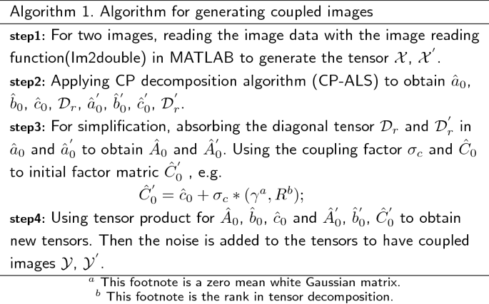

  

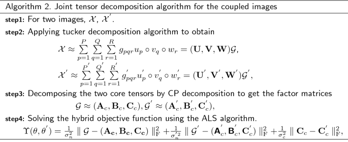
• b. Joint tensor decomposition of high dimensional coupled images

  For the actual high-dimensional images, a high dimensional coupled image decomposition algorithm is proposed. It is assumed that the coupling relationship between images is as follow:

  $$\begin{aligned} {{\mathbf {C}}}={\mathbf {C^{'}}}+\Gamma , \end{aligned}$$

  (28)

  where $\Gamma$ is an i.i.d. Gaussian matrix with variance of each element $\sigma _{c}^{2}$ and ${{\mathbf {C}}}^{'}$ has columns of given norm. If we disregard the coupling of the tensors, a common method to retrieve the CP models is to compress the data arrays, decomposing the compressed tensors, and then uncompress the obtained factors matrices, which is a more computationally efficient way.

  For a three-order tensor ${\mathcal {X}}\in {\mathbb {R}}^{I\times J\times K}$,the tucker decomposition is expressed as

  $$\begin{aligned} {\mathcal {X}}\approx \sum \limits _{p=1}^{P}\sum \limits _{q=1}^{Q}\sum \limits _{r=1}^{R}g_{pqr}u_{p}\circ v_{q}\circ w_{r} = \llbracket {\mathcal {G}};{{\mathbf {U}}},{{\mathbf {V}}},{{\mathbf {W}}} \rrbracket , \end{aligned}$$

  (29)

  where ${{\mathbf {U}}}\in {\mathbb {R}}^{I\times P}$,${{\mathbf {V}}}\in {\mathbb {R}}^{J\times Q}$, and ${{\mathbf {W}}}\in {\mathbb {R}}^{K\times R}$ are the factor matrices ,which are usually orthogonal. The positive integers P, Q, and R are the number of components (i.e., columns) in the factor matrices ${{\mathbf {U}}}$, ${{\mathbf {V}}}$, and ${{\mathbf {W}}}$, respectively. The tensor ${\mathcal {G}}\in {\mathbb {R}}^{P\times Q\times R}$ is called the core tensor. Tucker decomposition is a high-order principal component analysis, which represents a tensor as a core tensor multiplied by a matrix along each mode.

  If we assume two tensors are noiseless, i.e.

  $$ \begin{gathered} {\mathcal{X}} \approx \sum\limits_{{p = 1}}^{P} {\sum\limits_{{q = 1}}^{Q} {\sum\limits_{{r = 1}}^{R} {g_{{pqr}} } } } u_{p} ^\circ v_{q} ^\circ w_{r} = \left( {{\mathbf{U}},{\mathbf{V}},{\mathbf{W}}} \right) {\mathcal{G}}, \hfill \\ {\mathcal{X}^{\prime}} \approx \sum\limits_{{p = 1}}^{{P^{\prime}}} {\sum\limits_{{q = 1}}^{{Q^{\prime}}} {\sum\limits_{{r = 1}}^{{R{^{\prime}}}} {g{^{\prime}}_{{pqr}} } } } u{^{\prime}}_{p} ^\circ v{^{\prime}}_{q} ^\circ w{^{\prime}}_{r} = \left( {{\mathbf{U^{\prime}}},{\mathbf{V{^{\prime}}}},{\mathbf{W^{\prime}}}} \right){\mathcal{G}^{\prime}}, \hfill \\ \end{gathered} $$

  (30)

  In this section, we consider the decomposition algorithm of the coupled high dimensional images. The high dimensional image is decomposed into the low dimensional core tensor through the Tucker decomposition, and then decomposing the two core tensors by CP decomposition to get the factor matrices, the compressed CP models will reduce the cost and consumption of the calculation. There exists the relationship below.

  $$\begin{aligned} \begin{aligned} {\mathcal {G}}\approx ({{\mathbf {A}}}_{c},{{\mathbf {B}}}_{c},{{\mathbf {C}}}_{c}), {\mathcal {G}}^{'}\approx ({{\mathbf {A}}}_{c}^{'},{{\mathbf {B}}}^{'}_{c},{{\mathbf {C}}}^{'}_{c}), \end{aligned} \end{aligned}$$

  (31)

  The factor matrix of the original tensor can be solved by matrix multiplication with less computation.

  $$\begin{aligned} \begin{aligned} ({{\mathbf {U}}},{{\mathbf {V}}},{{\mathbf {W}}}){\mathcal {G}}=({{\mathbf {U}}}{{\mathbf {A}}}_{c},{{\mathbf {V}}}{{\mathbf {B}}}_{c},{{\mathbf {W}}}{{\mathbf {C}}}_{c}), {\mathbf {A=UA_{c}}},{\mathbf {B=VB_{c}}},{\mathbf {C=WC_{c}}} \end{aligned} \end{aligned}$$

  (32)

  It is assumed that the coupling relationship between noiseless tensors in the compressed space as

  $$\begin{aligned} {{\mathbf {W}}}{{\mathbf {C}}}_{c}={{\mathbf {W}}}^{'}{{\mathbf {C}}}^{'}_{c}+\Gamma \end{aligned}$$

  (33)

  However, if one tensor is noisy(i.e. ${\mathcal {Y}}$),there exists the similarity coupling in the compressed dimension

  $$\begin{aligned} {{\mathbf {C}}}_{c}={{\mathbf {C}}}^{'}_{c}+\Gamma _{c} \end{aligned}$$

  (34)

  where $\Gamma _{c}$ is a matrix of same dimensions as ${{\mathbf {C}}}_{c}$ and with Gaussian i.i.d. entries of variance. The hybrid objective function in the compressed space is modified to the following objective function, which can be solved using the ALS algorithm.

  $$\begin{aligned} \Upsilon (\theta ,\theta ^{'})=\frac{1}{\sigma _{n}^{2}}\parallel {\mathcal {G}}-({\mathbf {A_{c}},B_{c},C_{c}}) \parallel _{{\mathrm {F}}}^{2}+\frac{1}{\sigma _{n}^{'2}}\parallel {\mathcal {G}}^{'}-({\mathbf{A }}^{'}_{c},{\mathbf{B }}^{'}_{c},{{\mathbf {C}}}^{'}_{c}) \parallel _{{\mathrm {F}}}^{2}+\frac{1}{\sigma _{c}^{2}}\parallel {{\mathbf {C}}}_{c}-{{\mathbf {C}}}^{'}_{c} \parallel _{{\mathrm {F}}}^{2}, \end{aligned}$$

  (35)

  For the factorization of some coupled images, we expect that the factor matrices obtained by factorization algorithm can be shown by images. That means to minimize the objective function under the constraint of nonnegative conditions. The MU algorithm is usually used for nonnegative matrix factorization [10].

  

Experiments and results

The main idea of this paper is applying the above coupled data fusion algorithms to deal with the image. It is well known that the stored data values of images are ordinarily large. If the tensor decomposition algorithm is applied directly to the coupled image data, the error is a big problem, which makes us use the command Im2double in Matlab to scale the values to reduce the numerical error in program operation.

CIF-OPT algorithm

In this section, the coupled matrix tensor decomposition method is applied to multispectral and panchromatic images. The original images which are the low spatial resolution multispectral image located in Beijing, China and the corresponding high spatial resolution panchromatic image are as follows.

The experimental data are captured from Airborne Visible Infrared Imaging Spectrome-TER (AVIRIS) in Beijing. The AVIRIS data can provide 224 spectral segments with a spatial resolution of 20 m, covering a spectral range of $0.2\sim 2.4$ m, and its spectral resolution is 10 nm. The size of multispectral and panchromatic images of area I which are shown in Figs. 5 and 6 are $300\times 300\times 3$ and $300\times 300$ pixels respectively. The size of multispectral and panchromatic images of area II which are shown in Figs. 7 and 8 are $256\times 256\times 3$ and $256\times 256$ pixels respectively. The multispectral and panchromatic image data of area I are read and initialized by MATLAB, and stored as tensor ${\mathcal {X}}\in {\mathbb {R}}^{300\times 300\times 3}$ and matrix ${{\mathbf {Y}}}\in {\mathbb {R}}^{300\times 300}$. And the tensors of area II are generated in the same way.

Fig. 5

The multispectral image of area I

Fig. 6

The panchromatic image of area I

Fig. 7

The multispectral image of area II

Fig. 8

The panchromatic image of area II

According to the data generation of the CIF-OPT algorithm, the original data are sampled from the multispectral and panchromatic images, and the initial factor matrix is obtained by the ALS algorithm. Using the tensor product and the matrix multiplication to calculate the noiseless initial tensor and matrix. Without losing generality, we set the coupled factor matrix between tensor and matrix to ${{\mathbf {C}}}$. In order to study the performance of the algorithm better, experiments are carried out under different noise levels.

Adding noise to the obtained tensor ${\mathcal {X}}\in {\mathbb {R}}^{300\times 300\times 3}$ and the matrix ${{\mathbf {Y}}}\in {\mathbb {R}}^{300\times 300}$ after initializing the images, e.g.

$$\begin{aligned} {\mathcal {X}}^{'}= \llbracket {\mathbf {A,B,C}} \rrbracket +\eta {\mathcal {N}}\frac{\Vert \llbracket {\mathbf {A,B,C}} \rrbracket \Vert }{\Vert {\mathcal {N}}\Vert }, \end{aligned}$$

(36)

where ${\mathcal {N}}\in {\mathbb {R}}^{300\times 300\times 3}$ is the stochastic Gaussian noise tensor, $\eta$ is used to control the noise level. Similarly, the Gaussian noise is added to the matrix ${{\mathbf {Y}}}$, that is,

$$\begin{aligned} {{\mathbf {Y}}}^{'}={\mathbf {AV}}^{{\mathrm {T}}}+\eta {{\mathbf {N}}}\frac{\Vert {\mathbf {AV}}^{{\mathrm {T}}}\Vert }{\Vert {{\mathbf {N}}}\Vert }, \end{aligned}$$

(37)

where ${{\mathbf {N}}}\in {\mathbb {R}}^{300\times 3}$ is the stochastic Gaussian noise matrix, $\eta$ is used to control the noise level.

In this experiment, four different noise levels are set, which are 0, 0.1, 0.25, and 0.35 respectively. As the terminating condition of the CIF-OPT algorithm, it needs to be satisfied

$$\begin{aligned} \triangledown f=\frac{|f_{k+1}-f_{k}|}{f_{k}}\le 10^{-8}, \end{aligned}$$

(38)

where f is the objective function, in addition, the maximum number of function values and iteration number is set to $10^{4}$ and $10^{3}$ respectively. In the process of experiment, the termination condition of algorithm depends on the change of function value before and after iteration.

The main purpose of this section is to apply the CIF-OPT algorithm to the coupled multispectral and panchromatic images and the specific results are shown in Table 1. From Table 1, it can be seen that the CIF-OPT algorithm has the similar fusion effect for different images, which shows that the algorithm has a certain robustness. The fusion effect will not change dramatically as the vary of image order and data elements. Moreover, the number of iterations does not alter greatly with the increase of order, which proves the feasibility of decomposition for coupled images.

Table 1 Comparison of decomposition algorithms on different areas

The change from coupled data to the coupled image decomposition algorithm shows the iteration times and the maximum number of functions that CIF-OPT algorithm needs to convergence is larger than CMTF-OPT algorithm. The results are inevitable, because the coupled image needs to be initialized and converted to the coupled data to achieve the algorithm when the coupled image is decomposed. Therefore, the convergence of algorithm requires more iteration times. Accordingly, by observing the experiment of adding noise to the coupled image, it can be seen that the proposed algorithm can realize the decomposition of the coupled image, and the decomposition effect is better than the CMTF-OPT algorithm under the certain noise level. Consequently, the above results prove the feasibility of coupled image decomposition.

Another ACMTF algorithm for coupling image decomposition conducted the same noise level experiment for region I, and compared with CMTF-OPT algorithm. The results are shown in Fig. 9. It can be seen that ACMTF algorithm is superior to CMTF-OPT algorithm in different noise levels. Therefore, based on the same parameters and noise conditions, this paper conducts the same noise level experiment for another ACIF algorithm of coupled image, and compares the target function value, iteration times, error and other parameter results between the two algorithms. The fusion effect under different noise levels is shown in Fig. 10. Experimental results show that CIF-OPT algorithm is more effective than ACIF algorithm when the added noise is less than 0.2. This is different from the data fusion effect of the two algorithms in the coupled data, and with the increase of noise level, the performance of the two algorithms in the fusion effect is almost the same, which shows that the improved image decomposition algorithm does not have better advantages than CIF-OPT algorithm.

Fig. 9

Comparison of objective function values under different noise levels

Fig. 10

Comparison of objective function values under different noise levels

In this paper, the number of iterations required for algorithm convergence is compared as shown in Fig. 11. It can be seen from Fig. 11 that the number of iterations required for ACIF algorithm to converge is more than CIF-OPT algorithm in most cases, and the running time from reaching convergence condition to algorithm termination is longer when the algorithm is running. In order to comprehensively consider various factors, this paper calculates the fusion errors of the four algorithms to comprehensively compare the accuracy of the algorithm for data decomposition. See Fig. 12 for the specific results.

Fig. 11

Comparison of iteration times in different regions

Fig. 12

Comparison of the error values in different noise levels

Figure 12 shows that to some extent, the decomposition effect of the coupled image is better than that of the coupled data, but the error of the decomposition algorithm of the coupled data has a certain stability, and the error difference is lower than that of the decomposition algorithm of the coupled image. For the two algorithms of coupled image decomposition, when the noise level is lower than 0.25, the error value of the two algorithms is unstable, and the error value of Fig. 12 is small. Therefore, with the increase of noise level, the error value of CIF-OPT algorithm is very close to that of ACIF algorithm. So for the coupled image decomposition algorithm, CIF-OPT algorithm shows better fusion effect at low noise level, and the error difference and the number of iterations required for algorithm convergence are less.

The above algorithm is mainly based on the comparison of the result parameters of region I. We compare the iterations of the algorithm and the difference between the objective function values for two different regions based on CIF-OPT algorithm, and the results are shown in Figs. 13 and 14. It can be seen that there is no obvious linear relationship between the number of iterations and the image size. Because the magnitude of Fig. 14 is very small, the objective function values of the two regions are very close, that is to say, the function optimal value of CIF-OPT algorithm will not change significantly due to the difference of image size and pixel.

Fig. 13

The coupled image ${\mathcal {X}}$

Fig. 14

The coupled image ${\mathcal {X}}^{'}$

Based on the proposed CIF-OPT optimization algorithm, the multispectral images of the missing data coupled with the panchromatic image are restored. That is, all the data of the panchromatic image are known. The specific results of the algorithm are shown in Figs. 15 and 16. Where the missing data of this experiment occurred in area II and the recovered data is the transformed data, not the original image data. By observing the data curve recovered by the CIF-OPT algorithm, it is known that the data recovery effect of the coupled image with $25\%$ missing data is better than the effect of image with $50\%$ missing data. That is, the correlation between real value and estimated value is stronger when the percentage of missing data is $25\%$, and the linear slope is closer to 1.

Fig. 15

Data estimation with $25\%$ missing data

Fig. 16

Data estimation with $50\%$ missing data

Straightforward hybrid Gaussian coupled decomposition

We consider the straightforward hybrid Gaussian coupling model ${{\mathbf {C}}}={\mathbf {C^{'}}}+\Gamma$. And we select the small images inside the red frame as the uncoupled original tensors of Algorithm 1 in Fig. 17. The two CP models are generated by these images with dimensions $I=I^{'}=J=J^{'}= 30$, $K= K^{'}=3$ and $R= R^{'} = 8$, e.g. ${\mathcal {Y}},\mathcal {Y^{'}}$. Then through simplification and adding Gaussian noise and different coupling intensity to ${\mathcal {Y}},\mathcal {Y^{'}}$ to obtain the new tensors $\mathcal {{\overline{Y}}},\mathcal {\overline{Y^{'}}}$.The original tensor images are shown in Figs. 18 and 19. And the new tensor $\mathcal {{\overline{Y}}}$ is almost noiseless $\sigma _{n} =0.001$, while $\mathcal {\overline{Y^{'}}}$ has some noise $\sigma ^{'}_{n} =0.1$. The coupled images were generated by Algorithm 1, and decomposed by the ALS algorithm (i.e. Alg. 1) in [8]. Alg. 1 is applied to estimate the CP models under 400 different noise and coupling realizations. We also evaluate the total MSE on the ${{\mathbf {C}}}$ and ${\mathbf {C^{'}}}$ factors and the total MSE for an ALS algorithm. And the total MSE on a factor, for example the total MSE on ${{\mathbf {C}}}$ with $N_{r}$ different noise realizations is $(1/N_{r})\sum ^{K}_{k=1}\sum ^{R}_{r=1}\sum ^{N_{r}}_{n=1}({{\mathbf {C}}}_{kr}-\hat{{{\mathbf {C}}}}_{kr}^{n})^{2}$, where $\hat{{{\mathbf {C}}}}_{kr}^{n}$ is the factor estimated in the n-th noise realization.

Fig. 17

The uncoupled original image

Fig. 18

The coupled image ${\mathcal {Y}}$

Fig. 19

The coupled image ${\mathcal {Y}}^{'}$

Due to the different coupling intensity of the image, we used the above algorithms to decompose the image and get the mean square error of the factor matrix C for different coupling intensity. We can see that the factor matrix is generally better estimated by increasing the coupling density while applying a hard coupling(i.e. ${{\mathbf {C}}} = {\mathbf {C^{'}}}$) in Fig. 20, since more information comes from the clean tensor through the coupling. For a flexible coupling, instead of the mean square error decreases while $1/\sigma _{c}>10^{2}$. And in the interval $1/\sigma _{c}\in [10;10^{4}]$, the flexible coupling model has better estimation performance than the hard couplings. For $1/\sigma _{c}>10^{4}$, the flexible couplings works better than a hard coupling.

Fig. 20

Total MSE for the factors ${{\mathbf {C}}}$ and ${\mathbf {C^{'}}}$ with different algorithms

Compressed coupled decomposition

For high-dimensional images, the compressed data decomposition algorithm is adopted in this paper. The selected images are the Lena noised images which are as follows in Figs. 21 and 22. The tensors are generated by the following two images with dimensions $I=I^{'}=J=J^{'}= 256$, $K= K^{'}=3$ and $P =50$, $Q =40$. For the coupled compression decomposition algorithm of large images, the number of decomposed components is not well defined. Therefore, under the condition of the same coupling density $(1/\sigma _{c}=10^{3})$, we selected the best number of components based on the MSE on factor matrix ${{\mathbf {C}}}$. The experimental results are shown in Fig. 23, which showed that the mean square error of factor matrix is the smallest when $R=3$. So later in this paper, $R=3$ as the best number of components is used for other experiments. Factor matrices are generated by CP decomposition algorithm similarly to the previous example. The matrix ${{\mathbf {C}}}$ is coupled with factor matrix ${{\mathbf {C}}}^{'}$ with additive zero mean Gaussian noise of variance $\sigma _{c}^{2}$. Where

$$\begin{aligned} \sigma _{c}=\left| \frac{det({{\mathbf {C}}}^{'}-{{\mathbf {C}}})}{det(\gamma ,R)}\right| , \end{aligned}$$

(39)

and $\gamma$ is a zero mean white Gaussian matrix. The data array $\mathcal {{\overline{Y}}}$ is almost noiseless $\sigma _{n} =0.001$, while $\mathcal {\overline{Y^{'}}}$ has some noise $\sigma ^{'}_{n} =0.1$.We compare the performance of the coupled algorithm in the compressed space and the uncompressed space. Results for 20 iterations of the coupled algorithms are shown in Figs. 24 and 25. Compression was computed with randomized SVD from [41]. And initializations were given by two coupled uncompressed ALS with 1000 iterations, themselves initialized by decomposing images.

Fig. 21

The coupled image ${\mathcal {X}}$

Fig. 22

The coupled image ${\mathcal {X}}^{'}$

Fig. 23

Decomposition performance of three algorithms under different ranks

Fig. 24

Total MSE for the factors ${{\mathbf {C}}}$ and ${\mathbf {C^{'}}}$ in the compressed space

Fig. 25

Total MSE for the factors ${{\mathbf {C}}}$ and ${\mathbf {C^{'}}}$ in the uncompressed space

As shown in the picture, the compression and ALS algorithms show similar performance in the case of coupling, and the decomposition accuracy of the two algorithms decreases with the increase of the coupling density.

Then we study the relationship between noise and algorithm estimation performance. The SNR for ${\mathcal {Y}}$ is set to 22 dB, and it varies from 4 dB to 20 dB for ${\mathcal {Y}}^{'}$.Where

$$\begin{aligned} \begin{aligned} {\mathrm {SNR}}({\mathcal {Y}})=10log_{10}\frac{R(1+\sigma _{c}^{2})}{IJ\sigma _{n}^{2}}, {\mathrm {SNR}}({\mathcal {Y}}^{'})=10log_{10}\frac{R}{I^{'}J^{'}\sigma _{n}^{'2}}. \end{aligned} \end{aligned}$$

(40)

We compare the performance of the coupled algorithm in the compressed space and the uncompressed space, as well as standard ALS in the uncompressed space. Note that in Fig. 26, when the SNR < 18 dB, uncoupled ALS algorithm works better than the remaining two algorithms. As the noise level increases, for SNR > 18 dB, the uncoupled ALS algorithm decreases estimation performance in both coupled and compression cases.

Fig. 26

Reconstruction MSE of noisy factor ${\mathbf {C^{'}}}$ with different algorithms

On the run time of the algorithm, Figs. 27 and 28 show the clear difference in computation time between kinds of decomposition algorithms. We can see that the compression decomposition algorithm obviously saves time and cost compared to the uncompressed algorithm which may be rather slow. As the noise level increases, uncoupled ALS decreases estimation performance in both coupled and compression cases. In addition, hybrid coupling model is only verified in Gaussian condition to show its effectiveness and we will do other experiments in the future to demonstrate the versatility of the algorithm.

Fig. 27

Computation time in the compressed space

Fig. 28

Computation time in the uncompressed space

Conclusions

In this paper, we propose two algorithms for coupled image decomposition, which mainly utilize the CMTF-OPT algorithm and the flexible Bayesian model in the coupled data decomposition. For the proposed CIF-OPT algorithm, the corresponding experiments show that the effect of the coupled image decomposition under the influence of different noise is robust, and the fusion effect is better than the CMTF-OPT algorithm, which shows that the coupled images decomposition algorithm is feasible. In addition, because the expression of a phenomenon can be different from all kinds of data sets, the link set of data decomposition should be flexible. Therefore, this paper presents the modified flexible Bayesian model. From the experiments of it, we can easily see that the factor matrix could be estimated better by increasing the coupling density. And from the aspect of algorithm, the flexible coupling model has better estimation performance than the hard coupling models. Moreover, a coupled data compression scheme is derived from tensor images of large data sets. As the noise level increases, uncoupled ALS decreases estimation performance in both coupled and compression cases. On the run time of the algorithm, the compression decomposition algorithm obviously saves time and cost compared to the uncompressed algorithm. In fact, the image matrix is nonnegative. Therefore, when considering the coupled image decomposition algorithm, adding non negative constraints is our work in the future.

References

Sui J, Adali T, Yu Q, Calhoun V (2012) A review of multivariate methods for multimodal fusion of brain imaging data. J Neurosci Methods 204:68–81
Wang D, Zhou J, He K, Liu C (2009) Using tucker decomposition to compress color images. Int Congress Image Signal Process 1–9:1408–1412
Zhou P, Lu C, Lin Z, Zhang C (2016) Tensor factorization for low-rank tensor completion. IEEE Trans Image Process 27(3):1152–1163
Veganzones MA, Cohen JE, Farias RC, Chanussot J, Comon P (2016) Nonnegative tensor CP decomposition of hyperspectral data. IEEE Trans Geosci Remote Sens 54:2577–2588
Zhang K, Wang M, Yang SY, Jiao LC (2018) Spatial-spectral-graph-regularized low-rank tensor decomposition for multispectral and hyperspectral image fusion. IEEE J Sel Top Appl Earth Observ Remote Sens 11(4):1030–1040
Li H, Li WB, Han GN, Liu F (2018) Coupled tensor decomposition for hyperspectral pansharpening. IEEE Access 6:34206–34213
Lin CH, Fei M, Chi CY, Hsieh CH (2018) A convex optimization-based coupled nonnegative matrix factorization algorithm for hyperspectral and multispectral data fusion. IEEE Trans Geosci Remote Sens 56(3):1652–1667
Li S, Dian R, Fang L, Bioucas-Dias JM (2018) Fusing hyperspectral and multispectral images via coupled sparse tensor factorization. IEEE Trans Image Process 27:4118–4130
Li ST, Dian RW, Fang LY et al (2018) Fusing hyperspectral and multispectral images via coupled sparse tensor factorization. IEEE Trans Image Process 27(8):4118–4130
Cohen J, Farias RC, Comon P (2014) Fast decomposition of large nonnegative tensors. IEEE Signal Proc Lett 22:862–866
Shashua A, Levin A (2001) Linear image coding for regression and classification using the tensor-rank principle. Comput Vis Pattern Recognit 1:42–49
Aidini A, Tsagkatakis G, Tsakalides P (2019) Compression of high-dimensional multispectral image time series using tensor decomposition learning. in: IEEE EUSIPCOEUSIPCO
Astrid M, Lee SI, Seo BU (2018) Rank selection of Cp-decomposed convolutional layers with variational Bayesian matrix factorization. In: IEEE ICACTICACT
Bauckhage C (2007) Robust tensor classifiers for color object recognition. Int Conf Image Anal Recognit 4633:352–363
Hardie RC, Eismann MT, Wilson GL (2004) MAP estimation for hyperspectral image resolution enhancement using an auxiliary sensor. IEEE Trans Image Process 13:1174–1184
Wei Q, Dobigeon N, Tourneret JY (2016) Fast fusion of multi-band images based on solving a Sylvester equation. IEEE Trans Image Process 23:1632–1636
Akhtar N, Shafait F, Mian A (2015) Bayesian sparse representation for hyperspectral image super resolution. Proc IEEE Conf Comput Vis Pattern Recognit 12:3631–3640
Farias RC, Cohen JE, Comon P (2016) Exploring multimodal data fusion through joint decompositions with flexible couplings. IEEE Trans Signal Process 64:4830–4844
Huang YG, Cao LB, Zhang J, Pan L, Liu YY (2018) Exploring feature coupling and model coupling for image source identification. IEEE Trans Inf Forensics Secur 13(12):3108–3121
Banerjee A, Basu S, Merugu S (2006) Multi-way clustering on relation graphs. Siam Int Conf Data Mining 127:145–157
Yu FW, Wu XX, Chen JL, Duan LX (2019) Exploiting images for video recognition: heterogeneous feature augmentation via symmetric adversarial learning. IEEE Trans Image Process 28(11):5308–5321
Jiang TX, Huang TZ, Zhao XL, Deng LJ, Wang Y (2017) A novel tensor-based video rain streaks removal approach via utilizing discriminatively intrinsic priors. In: Proc. IEEE Conf. Comput. Vis. Pattern Recognit. pp 4057-4066
Zhang K, Wang M, Yang S, Jiao L (2018) Spectral-graph-regularized low-rank tensor decomposition for multispectral and hyperspectral image fusion. IEEE J Sel Topics Appl Earth Observ Remote Sens 11:1030–1040
Jiang TX, Huang TZ, Zhao XL, Ji TY, Deng LJ (2018) Matrix factorization for low-rank tensor completion using Framelet prior. Inf Sci 436–437:403–417
Bengua JA, Phien HN, Tuan HD, Do MN (2017) Efficient tensor completion for color image and video recovery: low-rank tensor train. IEEE Trans Image Process 26:2466–2479
Jia C, Shao M, Fu Y (2017) Sparse canonical temporal alignment with deep tensor decomposition for action recognition. IEEE Trans Image Process 26:738–750
Jia C, Fu Y (2016) Low-rank tensor subspace learning for RGB-D action recognition. IEEE Trans Image Process 25:4641–4652
Qian Y, Xiong F, Zeng S, Zhou J, Tang YY (2017) Matrix-vector non-negative tensor factorization for blind unmixing of hyperspectral imagery. IEEE Trans Geosci Remote Sens 55:1776–1792
Acar E, Kolda TG, Dunlavy DM (2011) All-at-once optimization for coupled matrix and tensor factorizations. Computing Research Repository-CORR
Qi L (2005) Eigenvalues of a real supersymmetric tensor. J Symb Comput 40:1302–1324
Carroll JD, Chang JJ (1970) Analysis of individual differences in multidimensional scaling via an n-way generalization of ”Eckart-Young” decomposition. Psychometrika 35:283–319
Harshman RA (1970) Foundations of the PARAFAC procedure: Models and conditions for an ”explanatory” multi-model factor analysis. In: Ucla Working Papers in Phonetics 16:1-84
Tucher LR (1963) Implications of factor analysis of three-way matrices for measurement of change. University of Wisconsin Press, Madison, pp 122–137
Singh AP, Kumar G, Gupta R (2008) Relational learning via collective matrix factorization. In: ACM SIGKDD international conference on knowledge discovery and data mining. pp 650-658
Wang Z, Wang S, Zhu Y (2016) Review of image fusion based on pulse-coupled neural network. Arch Comput Methods Eng 23(4):659–671
Veshki FG, Vorobyov SA (2017) Multi-focus image fusion using sparse representation and coupled dictionary learning. 1(1):1–25
Yuan Z, Feng LY, Hou CP, Kung SY (2017) Hyperspectral and multispectral image fusion based on local low rank and coupled spectral unmixing. IEEE Trans Geosci Remote Sens 55(10):5997–6009
Buchanan AM, Fitzgibbon AW (2005) Damped newton algorithms for matrix factorization with missing data. In: IEEE computer society conference on computer vision and pattern recognition. pp 316-322
Tomasi G, Bro R (2006) A comparison of algorithms for fitting the PARAFAC model. Comput Stat Data Anal 50:1700–1734
Ho C, Basdogan C, Srinivasan M. Numerical optimization: [M]. 2006.
Halko N, Martinsson PG, Tropp J (2011) Finding structure with randomness: probabilistic algorithms for constructing approximate matrix decompositions. SIAM Rev 53(2):217–288
Acknowledgements
The authors would like to thank the editors and anonymous reviewers. This work was partially supported by the National Natural Science Foundation of China under No. 51877144. This work was supported in part by MOST under contracts 109-2634-F-259-001—through Pervasive Artificial Intelligence Research (PAIR) Labs, Taiwan R.O.C.
Funding
This work was partially supported by the National Natural Science Foundation of China under No. 51877144.
Author information
Authors and Affiliations
Contributions
LL, ZT and JC contributed in the innovation ideas and theoretical analysis. XR and KHY helped to perform the analysis with constructive discussions and carry out experiments. All authors read and approved the final manuscript.
Corresponding authors
Ethics declarations
Competing interests
The authors declare that they have no competing interests.
Additional information
Publisher’s Note
Springer Nature remains neutral with regard to jurisdictional claims in published maps and institutional affiliations.
Rights and permissions
Open Access This article is licensed under a Creative Commons Attribution 4.0 International License, which permits use, sharing, adaptation, distribution and reproduction in any medium or format, as long as you give appropriate credit to the original author(s) and the source, provide a link to the Creative Commons licence, and indicate if changes were made. The images or other third party material in this article are included in the article's Creative Commons licence, unless indicated otherwise in a credit line to the material. If material is not included in the article's Creative Commons licence and your intended use is not permitted by statutory regulation or exceeds the permitted use, you will need to obtain permission directly from the copyright holder. To view a copy of this licence, visit http://creativecommons.org/licenses/by/4.0/.
About this article
Cite this article
Lu, L., Ren, X., Yeh, KH. et al. Exploring coupled images fusion based on joint tensor decomposition. Hum. Cent. Comput. Inf. Sci. 10, 10 (2020). https://doi.org/10.1186/s13673-020-00215-z
Received:
Accepted:
Published:
DOI: https://doi.org/10.1186/s13673-020-00215-z